Gambler's ruin in Astro and the accuracy of Gaussian approximation [1]

Recently, I was on a holiday trip with a friend, let’s call him Nathan. While not exactly a gambling addict, Nathan likes to buy scratchcards every now and then. One of his favourites is called Astro; most newspapers shops in France sell them for €2 a piece, and there exists 12 different versions, one for each astrological sign. While the sign itself does not affect the odds (at least I don’t believe so), it is a brilliant marketing strategy as it encourages you to buy a few more tickets and distribute them to your friends born under a different star than yours. Nathan is a Sagittarius, and that day he acquired a set of tickets, including an extra Aquarius one that he gifted to me. As it turned out, all but one of the set were loosers, the Aquarius one being the sole winner of a modest €6. Emboldened by this unexpected luck, I exchanged my gains for three more tickets to distribute among friends, keeping one Aquarius for myself. Again, all loosers but mine. This time I cashed out and stopped the gambling streak, much to Nathan’s dismay. I admit this is not a particularly exciting vacation story, but it got me thinking: what if I did not cashed out? How long could I have last by just reinvesting my gains, flying off Nathan’s initial €2 ticket?
The Astro distribution
Astro is a fairly transparent game: whoever takes the time to read the back of a ticket can learn all there is to know about the odds and possible profits. On mine, it read that 4,500,000 tickets were issued, among which 661,500 are winners for €2, 476,000 for €4, 150,000 for €6, 101,350 for €10, 45,000 for €20, 415 for €17T00, 8 for €1,000 and finally 3 extra lucky ones for €25,000. The figure below shows this gain distribution, with probabilities displayed in logarithmic scale for readability.
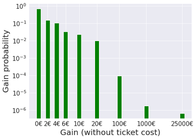
The expected gain of a ticket chosen uniformly at random (which I assume is how tickets are assigned to vendors) can be easily calculated from the above information and reads $\mathbb{E}[gain] = \sum_{x} x\mathbb{P}(gain=x) = 1.37$. After substracting the €2 cost of a ticket, the expected net payoff of a single Astro ticket is then $-0.63$. This makes perfect sense: the company that issues these tickets makes 63 cents on each, i.e about €2.3m in total.
In addition, we can also compute the variance with the formula $\sigma^2 = \mathbb{E}[gain^2] - \mathbb{E}[gain]^2$, which gives $\sigma\approx 20.67$.
Flight time
Going back to our initial question: how long can we defy the odds and keep “flying” from only the initial investment of €2? Let’s introduce some notations. We denote by $\left( g_t \right)_{t\in\mathbb{N}}$ a sequence of i.i.d samples drawn from the Astro distribution and let $\xi_t = 2 - g_t$ be the corresponding net loss, including the ticket price, and $$ X_t = \sum_{s=1}^t \xi_s $$ be the cumulative loss process. The more $X_t$ increases, the more losses the gambler suffers.
Note that the i.i.d assumption does not exactly hold: once a ticket is bought and scratched, it is removed from the pool of available tickets and cannot be acquired again, i.e. the true sampling is without replacement. We will see later that this only has a limited impact on the final result, which is quite intuitive: if you draw only a few samples, say a few dozens at most, with replacement, it is quite unlikely that you would sample twice the same among the $N=4,500,000$.
Our problem of “flight time” corresponds to studying the following random time: $$ \tau_{\alpha} = \inf \left\lbrace t\in\mathbb{N}, X_t \geq \alpha \right\rbrace, $$ which is a stopping time with respect to the natural filtration $\left(\mathcal{F}_t\right)_{t\in\mathbb{N}}$ induced by the process $X$, i.e. $\mathcal{F}_t=\sigma\left( X_s, 0\leq s\leq t\right)$ (this means $\left\lbrace \tau_{\alpha} \geq t\right\rbrace$ is an event in $\mathcal{F}_t$ for all $t\in\mathbb{N}$, i.e. one knows from the information available at time $t$ whether or not the stopping event occured or not). Indeed, reaching the threshold $\alpha=2$ for the cumulative loss $X_t$ is equivalent to reaching €0 wealth for a gambler who starts at €2 and keeps scratching Astro at every round, which we informally defined as the “flight time” above.
The Gaussian case
The reader versed in martingales will almost surely recognise this problem as an instance of gambler’s ruin. Indeed, the distribution of $\tau_{\alpha}$ can be fully explicited when the increments $\xi$ are Gaussian, in the limit of continuous time $t\in\mathbb{R}_+$ (instead of $t\in\mathbb{N}$). For completeness, we derive below this standard result using stochastic calculus.
We define the process $Z$ as
\begin{align*}
&dZ_t = \mu dt + \sigma dW_t\,,\\
&Z_0=0\,,
\end{align*}
where $\mu=0.63$, $\sigma=20.67$ and $W$ is a standard Brownian motion with respect to the filtration $\mathcal{F}$. Intuitively, we retrieve the discrete time model by the correspondence $dt\approx 1$ and $dW_t \approx \xi_t$. The loss process $Z$ can be more directly expressed as
$$
Z_t = \mu t + \sigma W_t\,,
$$
and the flight time in this context naturally becomes $\bar{\tau}_{\alpha} = \inf \left\lbrace t\in\mathbb{R}_+, Z_t \geq \alpha \right\rbrace$.
Of martingales and stopping times
Studying a stopping time can be quite hard, and coupling it with the right martingale is often the easiest approach. We recall here some elementary results on the interplay between martingales and stopping times. For convenience, we denote by $\mathcal{T}$ either $\mathbb{N}$ or $\mathbb{R}_+$ (the results presented below are essentially unchanged by moving to the continuous or discrete time setting).
First, a process $\left(M_t\right)_{t\in\mathcal{T}}$ is a martingale with respect to a filtration $\left(\mathcal{F}_t\right)_{t\in\mathcal{T}}$ if for all $t\in\mathcal{T}$, $M_t$ is $\mathcal{F}_t$-adapted, integrable and satisfies the equality $$ \forall s\in\mathcal{T},\ \mathbb{E}\left[M_{t+s}\mid \mathcal{F}_t\right] = M_t\,. $$
Intuitively, this means a martingale represents a fair game: if $M_t$ represents a fictitious amount of wealth for the player at time $t$, then $M_t$ is fully known from the information available at time $t$ ($\mathcal{F}_t$-adapted) and the estimation of future wealth is exactly $M_t$ (by contrast, a loosing game would satisfy $\mathbb{E}\left[M_{t+s}\mid \mathcal{F}_t\right] \leq M_t$; such processes are called supermartingales). This property is sometimes referred to as martingales being “constant in expectation”.
The crucial property of martingales for the study of stopping times is called Doob’s optional stopping theorem: for any $\mathcal{F}$-stopping time, the stopped process $\left(M_{t\wedge \tau}\right)_{t\in\mathcal{T}}$ is also a $\mathcal{F}$-martingale, where $t\wedge \tau$ represents the minimum between $t$ and $\tau$. By taking the expectation of the above equality applied to the stopped martingale, we obtain the following identity: $$ \forall t\in\mathcal{T},\ \mathbb{E}\left[M_{t\wedge \tau}\right] = \mathbb{E}\left[M_0\right]\,. $$
Ideally, we would like to have the simpler equality $\mathbb{E}\left[M_{\tau}\right] = \mathbb{E}\left[M_0\right]$ instead, which depending on the exact expression of $M$ can reveal key properties of $\tau$ (expectation or higher moments, density function…). It is therefore tempting to take the limit $t\rightarrow +\infty$ in the above and hope that one can swap limit and expectation. This holds under a variety of technical assumptions. A simple argument, which is enough for our purpose, is to use the dominated convergence theorem, provided $M_{t\wedge \tau}$ can be bounded by an integrable random variable independent of $t$.
Building the right martingale
For $\lambda\in\mathbb{R}$, we define $$ M^\lambda_t = \exp\left( \lambda W_t - \frac{\lambda^2}{2}t\right)\,. $$ It is a standard result in stochastic calculus that $M^\lambda$ defines a $\mathcal{F}$-martingale (it follows from the expression of the moment generating function of the standard Gaussian distribution coupled with the fact that the law of $W_t$ is $\mathcal{N}\left(0, t\right)$). Moreover, it can be rewritten as $M^\lambda_t = \exp\left( \frac{\lambda}{\sigma} Z_t - (\frac{\lambda^2}{2} + \frac{\lambda \mu}{\sigma})t\right)$. The reason why this is the “right” martingale will become apparent soon: it will help us compute exponential moments of $\bar{\tau}_{\alpha}$, also known as the Laplace transform, which fully characterises its distribution.
Note that $t\mapsto Z_t$ is (almost-surely) continuous (since $t\mapsto W_t$ is), and therefore $Z_{\bar{\tau}_{\alpha}}=\alpha$ on the event $\left\lbrace \bar{\tau}_{\alpha} < \infty\right\rbrace$. As a consequence, it is straightforward to control $M^{\lambda}_{t\wedge \bar{\tau}_{\alpha}}$ in the following way: $$ \lvert M^\lambda_{t\wedge \bar{\tau}_{\alpha}} \rvert \leq e^{\frac{\lambda}{\sigma} \max(Z_{t\wedge \bar{\tau}_{\alpha}}, 0) } \leq e^{\frac{\lambda \alpha}{\sigma}}\,, $$ which allows to use the dominated convergence theorem as discussed above. Therefore, Doob’s optional stopping theorem yields: $$ \mathbb{E}[M^\lambda_{\bar{\tau}_{\alpha}}]=\mathbb{E}[e^{\frac{\lambda \alpha}{\sigma} - (\frac{\lambda^2}{2} + \frac{\lambda \mu}{\sigma})\bar{\tau}_{\alpha}}]=1\,. $$ After rearranging termes, we obtain the identity $$ \mathbb{E}[e^{-(\frac{\lambda^2}{2} + \frac{\lambda \mu}{\sigma})\bar{\tau}_{\alpha}}] = e^{-\frac{\lambda \alpha}{\sigma}}\,. $$ This is almost the Laplace transform of $\bar{\tau}_{\alpha}$, which we define for $\beta>0$ as $\mathbb{E}[e^{-\beta \bar{\tau}_{\alpha}}]$. Since $\bar{\tau}_{\alpha}$ is nonnegative, this Laplace transform fully characterises its distribution. Solving $\beta = \frac{\lambda^2}{2} + \frac{\lambda \mu}{\sigma}$ in terms of $\lambda$ yields $\lambda=-\frac{\mu}{\sigma} + \sqrt{\frac{\mu^2}{\sigma^2} + 2\beta}$ for $\lambda\geq 0$, i.e. $$ \mathbb{E}[e^{-\beta \bar{\tau}_{\alpha}}] = e^{\frac{\alpha \mu}{\sigma^2}\left(1 - \sqrt{1 + \frac{2\sigma^2 \beta}{\mu^2}}\right)} \,. $$
Besides characterising the distribution, the Laplace transform is also useful to compute the moments. Indeed, by differentiating w.r.t. $\beta$ (we differentiate inside the expectation since $e^{-\beta \bar{\tau}}\leq 1$ almost surely), we have that $$ -\frac{\partial}{\partial \beta} \mathbb{E}[e^{-\beta \bar{\tau}_{\alpha}}]\bigg|_{\beta=0} = \mathbb{E}[\bar{\tau}_{\alpha}] = \frac{\alpha}{\mu}\,. $$
After all these calculations, let’s take a step back to reflect on what this result means. On average, a gambler reaches the critical threshold $\alpha=2$ after $\frac{\alpha}{\mu}=\frac{2}{0.63}\approx 3.17$ rounds. This is, perhaps quite surprisingly, very intuitive: if you start from €2 and loose on average $63$ cents each time you play, it should take you a bit more than 3 rounds to consume your initial €2. The above shows that this back-of-the-envelope calculation is exact in the continuous time Gaussian case. Moreover, this result is independent of the variance $\sigma^2$.
Nice! Does this mean that I can play thrice at the cost of a single ticket most of the time?
Not at all! It is important to make the distinction here between mean and median flight times. Intuitively, the distribution of flight time $\bar{\tau}_{\alpha}$ should be quite asymmetrical around its mean: events where large gains are made early (e.g. first ticket yields €100) will result in very large flight times but remain quite rare, while events of “early crashes” (the first few tickets are loosers) are much more frequent. Therefore, the median flight time, i.e. the majority of flight times are below it, should be less than the mean flight time, which is driven upwards by the “early luck” outliers. This type of distribution is called right-skewed.
Flight time distribution in the Gaussian case
The expression of the Laplace transform $\mathbb{E}[e^{-\beta \bar{\tau}_{\alpha}}]$ reveals that $\bar{\tau}_{\alpha}$ follows an Inverse Gaussian distribution $IG\left(\frac{\alpha}{\mu}, \frac{\alpha^2}{\sigma^2}\right)$, the density of which is given by:
$$
p_{\bar{\tau}_{\alpha}}(t) = \sqrt{\frac{\alpha^2}{2\pi \sigma^2 t^3}} \exp\left(-\frac{\left(\mu t - \alpha\right)^2}{2\sigma^2 t} \right)\,.
$$
Its mean and variance are given respectively by
\begin{align*}
\mathbb{E}\left[\bar{\tau}_{\alpha}\right]&= \frac{\alpha}{\mu} \approx 3.17\,,\\
\mathbb{V}\left[\bar{\tau}_{\alpha}\right]&= \frac{\alpha \sigma^2}{\mu^3} \approx 58.46^2\,.
\end{align*}
We plot below this density for the Astro parameters ($\mu=0.63, \sigma=20.67, \alpha=2$), as well as the mean, standard deviation (SD), and the 5th, 25th, 50th (median), 75th and 95th percentiles. This distribution appears to be significantly right-skewed: even the 95th percentile is below the mean ($2.14$ versus $3.17$). In other words, according to the Gaussian approximation, it is really unlikely (less than 5% chance) that your flight time will be above 2 rounds, even though the mean flight time is above 3!
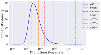
| mean | SD | 5th | 25th | 50th | 75th | 95th | |
|---|---|---|---|---|---|---|---|
| IG approximation | 3.17 | 58.46 | 0.00 | 0.01 | 0.02 | 0.09 | 2.14 |
What’s next?
Next time, we will talk about the flight time for the true Astro distribution, rather than under the Gaussian approximation. Deriving a closed-form expression for the distribution of $\tau_{\alpha}$ is more intricate, so simulations will prove handy.
License
Copyright 2022-present Patrick Saux.