Gambler's ruin in Astro and the accuracy of Gaussian approximation [2]

Assessing the quality of the Gaussian approximation
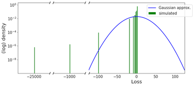
In the previous post, we calculated the distribution of the flight time of the cumulative Gaussian loss process $Z_t=\mu t + \sigma W_t$, that is $\bar{\tau}_{\alpha} = \inf \left\lbrace t\in\mathbb{R}_+, Z_t \geq \alpha \right\rbrace$, and shown that it was equal to the inverse Gaussian distribution $IG\left(\frac{\alpha}{\mu}, \frac{\alpha^2}{\sigma^2}\right)$. In the game of Astro though, the loss distribution for scratching a card is far from Gaussian: it is discrete, asymmetrical, with pronounced skewness towards small losses. The figure below shows the difference between the true Astro distribution (in green) and its Gaussian approximation $\mathcal{N}(\mu, \sigma^2)$ (in blue), with $\mu=0.63$ and $\sigma=20.67$.
It is insightful to look at the empirical estimation of $\mu$ and $\sigma$ under both the true Astro model and its Gaussian approximation. We define the standard (unbiased) sample estimators
\begin{align*}
&\widehat{\mu}_t = \frac{1}{t}\sum_{s=1}^t \xi_s \,,\\
&\widehat{\sigma}^2_t = \frac{1}{t-1}\sum_{s=1}^t \left(\xi_s - \widehat{\mu}_t\right)^2 \,,
\end{align*}
and report below the median (25th - 75th percentile in shaded area) of 10 independent replications of $\widehat{\mu}_t$ and $\widehat{\sigma}_t$ for $t$ ranging from 2 to 4,500,000, where $\xi$ is sampled from the Astro distribution (in green) and the Gaussian approximation (in blue).
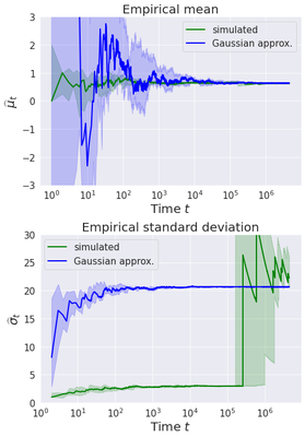
For the mean estimation, as expected, $\widehat{\mu}_t$ converges to the true expected value $\mu=0.63$, with higher dispersion in the Gaussian case. For the variance estimation, $\widehat{\sigma}_t$ seems to converge quite fast to the true value $\sigma=20.67$ in the Gaussian case, but remains much lower in the Astro model until $t\approx 10^5$, before suddenly jumping to values around $\widehat{\sigma}_t\approx 20$. This is actually quite intuitive: the high variance of the Astro distribution is driven by the outlier gains, in particular 1,000 and 25,000, which occur with very small probability. Before $t\approx 10^5$, the samples $\xi_1, \dots, \xi_t$ used in $\widehat{\sigma}_t$ do not contain such outliers, thus estimating a seemingly low variance. In other words, the sample variance in the Astro model is subject to higher variability than in the Gaussian case, which hints at larger higher order moments (skewness, kurtosis…) in the Astro case. We confirm this intuition with a direct calculation, based on the formulae:
\begin{align*}
&skewness = \frac{\mathbb{E}\left[\left(\xi-\mu\right)^3\right]}{\sigma^{\frac{3}{2}}}\,,\\
&excess\ kurtosis = \frac{\mathbb{E}\left[\left(\xi-\mu\right)^4\right]}{\sigma^{2}} - 3\,.
\end{align*}
| $\mu$ | $\sigma$ | skewness | excess kurtosis | |
|---|---|---|---|---|
| Astro | 0.63 | 20.67 | -1180 | 1426486 |
| Gaussian | 0.63 | 20.67 | 0 | 0 |
Simulated flight time
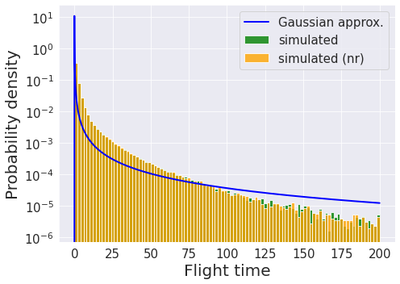
Contrary to the continuous time Gaussian case $\bar{\tau}_{\alpha}$, computing $\tau_{\alpha}=\inf\left\lbrace t\in\mathbb{N}, X_t \geq \alpha\right\rbrace$ in closed-form for the true Astro distribution is a priori intricate. However, it is straightforward to simulate random walks following the Astro distribution and therefore to estimate $\tau_{\alpha}$ by the Monte Carlo method. The result of 100 millions independent replications are reported below against the inverse Gaussian distribution coming from the Gaussian approximation model.
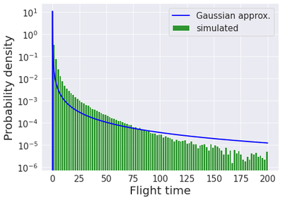
The simulation reveals that the inverse Gaussian approximation underestimates the probability of small flight times and overestimates that of longer ($>100$) flight times. In other words, the inverse Gaussian approximation does not account properly for the high risk of early crash. We report mean, standard deviation and percentiles of $\tau_{\alpha}$ and $\bar{\tau}_{\alpha}$, i.e. under both the simulated Astro and the inverse Gaussian models (95% confidence intervals for the simulated statistics are calculated by bootstrap with 400 independent replications).
| mean | SD | 5th | 25th | 50th | 75th | 95th | |
|---|---|---|---|---|---|---|---|
| Astro (simulated) $\tau_{\alpha}$ | 3.20 [3.15 ; 3.27] |
60.8 [39.9 ; 78.4] |
1.0 [1.0 ; 1.0] |
1.0 [1.0 ; 1.0] |
1.0 [1.0 ; 1.0] |
2.0 [2.0 ; 2.0] |
11.0 [11.0 ; 11.0] |
| IG approximation $\bar{\tau}_{\alpha}$ | 3.17 | 58.46 | 0.00 | 0.01 | 0.02 | 0.09 | 2.14 |
The expectation and variance of $\tau_{\alpha}$ are, perhaps surprisingly, well estimated in the inverse Gaussian model; in fact, it is statistically plausible that $\mathbb{E}\left[\tau_{\alpha}\right] = \mathbb{E}\left[\bar{\tau}_{\alpha}\right]$ ($3.17 \in [3.15 ; 3.27]$) and $\mathbb{V}\left[\tau_{\alpha}\right] = \mathbb{V}\left[\bar{\tau}_{\alpha}\right]$ ($58.46\in [39.9 ; 78.4]$). This is actually somewhat intuitive: remember the expectation of $IG\left(\frac{\alpha}{\mu}, \frac{\alpha^2}{\sigma^2}\right)$ is $\frac{\alpha}{\mu}$, which depends only on the threshold $\alpha$ and the expectation $\mu$ of the Astro random walk, not on higher moments which are crucially underestimated by the Gaussian approximation. On the contrary, quantiles are poorly estimated by the Gaussian model, partly because of the continuous time (quantiles in the discrete time Astro model cannot be less than 1, whereas the inverse Gaussian distribution puts a lot of mass on $[0, 1]$).
Conclusion
The inverse Gaussian approximation based on continuous time martingale arguments offers an analytical expression that tracks quite accurately the expected flight time of scratching Astro cards. In a sense, this is an empirical manifestation of the ubiquitous property that Gaussian distributions are limits of distributions with finite variance (central limit theorem, Donsker’s theorem on random walks…). This sort of approximation is numerically consistent in expectation. but much less so for other statistics, e.g. the quantiles. Moreover, let’s emphasise again the difference in interpretation between mean and median: the expected flight time $\mathbb{E}\left[\tau_{\alpha}\right]\approx 3.17$ is driven upwards by unlikely events of large magnitude; the most likely outcome of scratching Astro cards is to loose 2€ all at once!
Finally, you may check out the code used for the simulation and figures in this repo.
What’s next?
Is this the best we can do? It turns out that the Astro random walk is actually a special case where the martingale arguments developed for the inverse Gaussian approximation do hold in discrete time! We will detail this in the next post and derive in particular the exact expression of $\mathbb{E}\left[\tau_{\alpha}\right]$. Spoiler: the inverse Gaussian approximation was indeed not so bad in expectation!
Bonus
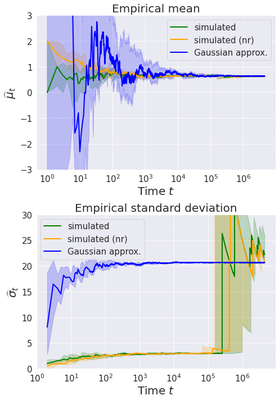
In this first post, we mentioned a subtlety of the sampling mechanism in Astro: bought tickets are effectively removed from the pool of available tickets, and therefore sampling from the Astro distribution should be done without replacement. Intuitively though, this should be negligible since the typical flight time is much smaller than the total amount of tickets (4,500,000). To convince ourselves, we report below figures on mean and variance estimation as well as the distribution of flight time under sampling with no replacement (nr) and visually verify that they are similar to their counterparts with replacement.
Cheers!
P.S: kudos to Pierre Bauvin for proofreading and for asking that I write it all down in the first place!
License
Copyright 2022-present Patrick Saux.